`drcmd`: Doubly-Robust Causal Inference with Missing Data

Keith Barnatchez
Johns Hopkins University
Department of Biostatistics
kbarnat1@jh.edu

Griffin DesRoches
University of Massachusetts, Amherst

Note: Package is still in development. Exercise caution while using this package until it’s been fully developed, and please check back frequently for updates.

Introduction

The drcmd R package performs semi-parametric efficient estimation of causal effects of point exposures in settings where the data available to the researcher is subject to missingness. By implementing methods from semi-parametric theory and missing data (see, e.g. Robins, Rotnitzky, and Zhao (1994) and Kennedy (2022)), drcmd accommodates general patterns of missing data, while enabling users to estimate nuisance functions with flexible machine learning methods. drcmd automatically determines the missingness patterns present in user-supplied data, and provides information on assumptions that must hold regarding the missingness mechanisms in order for point estimates and inferences to be valid. By accommodating general patterns of missingness, drcmd serves as a centralized library for researchers aiming to perform causal inference with missing data.

The use of doubly-robust methods for performing causal inference of point exposures on outcomes of interest has surged over the past decade, and numerous software packages have been developed for implementing these estimators. While these packages are well-suited for use on complete, missingness-free data, leading statistical software packages provide little to no support for missing data. The lack of a centralized package for performing doubly-robust causal inference has functioned as a severe impediment for researchers, as missing data is ubiquitous in real-world data, and the specific patterns of missingness can greatly vary across applications. drcmd addresses this shortcoming by providing a single R package for performing doubly-robust causal inference in the presence of general missing data patterns.

Getting started

Installation

drcmd is hosted on GitHub. The latest version be installed through the devtools package:

devtools::install_github('keithbarnatchez/drcmd')

Illustrative example

To illustrate the use of the drcmd package, we will consider a missing data problem where the outcome of interest $Y$ is missing at random conditional on measured covariates. We will assume a cheap, noisy proxy measurement for $Y$, denoted $Y^*$, is available for all subjects but not predictive of missingness (so that it is not necessary to satisfy the MAR assumption), resulting in the following simple data generating process:

$$\begin{aligned} X & \sim N(0,1) \ \ \ \ \ \ &\text{(Covariates)} \\ A|X & \sim \text{Bernoulli}(p = \text{logit}^{-1}(X)) \ \ \ \ \ \ &\text{(Treatment)} \\ Y|A,X & \sim N(\mu=A + X + AX, \sigma^2=1) \ \ \ \ \ \ &\text{(Outcome)} \\ Y^* & = Y + \varepsilon, \ \varepsilon \sim N(\mu=0,\sigma^2 = 1/4) \ \ \ \ \ \ &\text{(Outcome Proxy)} \\ R &\sim \text{Bernoulli}(\text{logit}^{-1}(X)) \ \ \ \ \ \ &\text{(Complete case Indicator)} \\ \end{aligned}$$$Y$ is only available when the complete case indicator $R=1$, and the missing at random assumption implies $Y \perp R | X$. We simulate data from this model below:

n <- 1e3
X <- rnorm(n) ; A <- rbinom(n,1,plogis(X)) ; Y <- rnorm(n) + A + X + A*X
Ystar <- Y + rnorm(n)/2 ; R <- rbinom(n,1,plogis(X)) ; X <- as.data.frame(X)
Y[R==0] <- NA # Make Y NA if R==0

df <- data.frame(Y=Y,A=A,X=X,Ystar=Ystar,R=R)
head(df)

##           Y A            X      Ystar R
## 1        NA 0 -1.400043517 -1.7855709 0
## 2        NA 0  0.255317055 -0.3332133 0
## 3        NA 0 -2.437263611 -4.6215099 0
## 4 -1.539838 0 -0.005571287 -2.6864287 1
## 5        NA 0  0.621552721  0.4344233 0
## 6        NA 1  1.148411606  4.5822774 0

The main function from the drcmd package is drcmd(). The core arguments are Y, A and X, representing the outcome, binary treatment and covariates. Users can optionally specify proxy variables W that are (i) predictive of the missing variables, (ii) possibly influence the missingness mechanism, and (iii) wouldn’t be involved in the causal analysis under the presence of complete data. Such variables commonly arise in semi-supervised inference, where cheap proxies are often available for expensive-to-measure variables. In our running example, we have that $Y^*=W$. In practice, $W$ can be multi-dimensional when multiple proxies are available. W defaults to NA when not specified by the user, consistent with settings where proxies are not available.

Missing data are allowed in the outcome, treatment, and covariates (including any subset of covariates), as well as any combination of the three. The only requirement for running drcmd is that there exists at least one variable that is never missing, either in Y, A, X, W. drcmd detects missingness patterns in the data and automatically creates a variable R, where R=1 if the observation is a complete-case and R=0 if the observation is missing. Note that this does not guarantee identifiability of the causal estimands $\mathbb{E}[Y(1)]$ or $\mathbb{E}[Y(0)]$. The validity of the resulting estimates hinges on the MAR assumption holding, a crucial problem-specific determination.

Along with specifying variables, users must specify means by which to estimate all nuisance functions. All nuisance functions are estimated through a Super Learner (a stacking algorithm) using the SuperLearner package. There are 4 nuisance functions that are fit by drcmd, for $a = 0,1$:

$$\begin{aligned} &1. \ m_a(X) = \mathbb{E}(Y|A=a,X) \\ &2. \ g_a(X) = \mathbb{P}(A=a|X) \\ &3. \ r(Z) = \mathbb{P}(R=1|Z) \\ &4. \ \varphi_a(Z) = \mathbb{E}(\chi_a(X,A,Y) | Z, R=1), \end{aligned}$$

where $\chi_a(X) = m_a(X) + \frac{I(A=a)}{g_a(X)}(Y-m_a(X))$ is the pseudo-outcome formed by the efficient influence function for estimating the counterfactual mean functional $\mathbb{E}[\mathbb{E}(Y|A=a,X)]$, and $Z$ collects all variables that are never subject to missingness (and are always available, regardless of whether $R=1$ or $R=0$). drcmd automatically determines the variables comprising $Z$.

Users can specify learners for each nuisance function through the nuisance-specific arguments below, or set a common library for all of them through default_learners. A nuisance-specific argument overrides default_learners for that function.

Argument	Nuisance function	Role
m_learners	$m_a(X) = \mathbb{E}(Y\mid A=a,X)$	Outcome regression
g_learners	$g_a(X) = \mathbb{P}(A=a\mid X)$	Treatment propensity score
r_learners	$r(Z) = \mathbb{P}(R=1\mid Z)$	Complete-case (missingness) propensity score
po_learners	$\varphi_a(Z)$	Pseudo-outcome regression
default_learners	—	Library applied to any nuisance not given its own argument

Each argument takes a vector of SuperLearner library names, using the same syntax one passes directly into SuperLearner. To see the base libraries available, users can run get_sl_libraries():

drcmd::get_sl_libraries()

##  [1] "SL.bartMachine"      "SL.bayesglm"         "SL.biglasso"        
##  [4] "SL.caret"            "SL.caret.rpart"      "SL.cforest"         
##  [7] "SL.earth"            "SL.gam"              "SL.gbm"             
## [10] "SL.glm"              "SL.glm.interaction"  "SL.glmnet"          
## [13] "SL.ipredbagg"        "SL.kernelKnn"        "SL.knn"             
## [16] "SL.ksvm"             "SL.lda"              "SL.leekasso"        
## [19] "SL.lm"               "SL.loess"            "SL.logreg"          
## [22] "SL.mean"             "SL.nnet"             "SL.nnls"            
## [25] "SL.polymars"         "SL.qda"              "SL.randomForest"    
## [28] "SL.ranger"           "SL.ridge"            "SL.rpart"           
## [31] "SL.rpartPrune"       "SL.speedglm"         "SL.speedlm"         
## [34] "SL.step"             "SL.step.forward"     "SL.step.interaction"
## [37] "SL.stepAIC"          "SL.svm"              "SL.template"        
## [40] "SL.xgboost"          "SL.hal9001"

This list includes SL.hal9001, a wrapper for the highly-adaptive LASSO (HAL). Users can additionally create custom libraries, and are encouraged to consult the SuperLearner package documentation for further details.

Cautionary note: weighted regressions

The nuisance functions $m_a$ and $g_a$ are estimated with regressions that add weights $R/\mathbb{P}(R=1|Z)$ to the underlying loss functions. In turn, libraries that do not support (or ignore) weights will tend to yield biased estimates. Users are encouraged to ensure all libraries used support weights.

Using drcmd

Calling the drcmd function

Below we demonstrate an example call of drcmd(), which requires users to provide an outcome Y, binary treatment A, covariate dataframe X, and SuperLearner libraries. We make use of the default_learners argument to specify SuperLearner libraries for all nuisance functions, estimating each through an ensemble of generalized linear models (GLMs) and generalized additive models (GAMs).

res <- drcmd::drcmd(Y=Y, A=A, X=X,
             default_learners=c('SL.glm','SL.gam'),
             quiet=FALSE)

To make use of the additional proxy variable, we can simply specify the W argument in the call to drcmd(). In general, W can be multidimensional. In our running example, we have that $Y^*=W$.

res <- drcmd::drcmd(Y=Y, A=A, X=X, W=data.frame(Ystar),
             default_learners=c('SL.gam'))

Users can specify specific learners through nuisance-specific arguments, which will overwrite the learners specified in default_learners for that particular nuisance function if default_learners is specified. For example, to estimate the pseudo-outcome regression through GAMs, and all other nuisance functions with a Super Learner ensemble of GLMs and splines, we can make the following call to drcmd():

res <- drcmd::drcmd(Y=Y, A=A, X=X,
             default_learners=c('SL.glm','SL.gam'),
             po_learners = 'SL.gam')

Alternatively, one can omit specification of default_learners entirely, provided learners are specified for each nuisance function:

res <- drcmd::drcmd(Y=Y, A=A, X=X,
             m_learners = c('SL.glm','SL.gam'), 
             g_learners = 'SL.mean',
             r_learners = 'SL.glm.interaction',
             po_learners = c('SL.gam','SL.hal9001'))

Outputting results

Users can view a summary of the estimation procedure by calling the summary() function, which provides point estimates, standard errors and 95% CIs for main causal estimands. By default, drcmd obtains estimates of $\mathbb{E}[Y(1)]$, $\mathbb{E}[Y(0)]$, and the average treatment effect (ATE) $\mathbb{E}[Y(1)-Y(0)]$. When the outcome is binary, drcmd additionally reports the causal risk ratio $\mathbb{E}[Y(1)]/\mathbb{E}[Y(0)]$ and odds ratio. Standard errors for these estimands are obtained via the delta method (see the Technical Details section).

summary(res)

## ======================================================================
##                         Summary of drcmd results                      
## ======================================================================
## Estimand            Estimate           SE                     95% CI
## ----------------------------------------------------------------------
## ATE:                   1.098        0.119             [0.864, 1.331]
## E[Y(1)]:               1.116        0.103             [0.915, 1.317]
## E[Y(0)]:               0.018        0.090            [-0.158, 0.194]
## ----------------------------------------------------------------------
## Variables with missingness (U): Y
## Variables without missingness (Z): X, A
## ----------------------------------------------------------------------
## Validity of results requires causal assumptions to hold,
## as well as the assumption that U is independent of R given Z

Extracting output

After running drcmd(), numerous objects are stored within the resulting output, including

• results: A list containing (i) parameter estimates stored in a dataframe named estimates, (ii) standard errors stored in a dataframe named ses, and (iii) nuisance function estimates stored in a dataframe named nuis
• params: A list containing all parameter values used by drcmd()
• R: Binary complete case indicator, where 1 denotes a complete case
• U: Names of variables with partially missing values
• Z: Names of variables with no missing values

Users can obtain a detailed summary by specifying detail=TRUE in the summary function:

summary(res,detail=TRUE)

## ======================================================================
##                         Summary of drcmd results                      
## ======================================================================
## Estimand            Estimate           SE                     95% CI
## ----------------------------------------------------------------------
## ATE:                   1.098        0.119             [0.864, 1.331]
## E[Y(1)]:               1.116        0.103             [0.915, 1.317]
## E[Y(0)]:               0.018        0.090            [-0.158, 0.194]
## ----------------------------------------------------------------------
## Variables with missingness (U): Y
## Variables without missingness (Z): X, A
## ----------------------------------------------------------------------
## Validity of results requires causal assumptions to hold,
## as well as the assumption that U is independent of R given Z
## ----------------------------------------------------------------------
## Number of cross-fitting folds (k): 1 
## Outcome regression nuisance learners: SL.glm SL.gam 
## Propensity score nuisance learners: SL.glm SL.gam 
## Missingness nuisance learners: SL.glm SL.gam 
## Pseudo-outcome nuisance learners: SL.glm SL.gam 
## Estimation method: augmented complete case one-step

Additional parameters

Cross-fitting

While not enabled by default, users can estimate parameters through cross-fitting by setting the k argument to the desired number of folds. By default, drcmd uses a single fold. Cross-fitting is encouraged when the user specifies nuisance learners that cover complex function classes, such as random forests. See the technical details section for more information on the rationale behind and implementation of cross-fitting.

When k > 1, the folds are independent and can be fit concurrently by setting parallel=TRUE, which distributes them across cores via parallel::mclapply (not supported on Windows). Separately, the cv_folds argument controls the number of cross-validation folds SuperLearner uses internally for model selection within each fit (default 5); lowering it speeds up estimation at some cost to learner selection.

res <- drcmd::drcmd(Y=Y, A=A, X=X,
             default_learners='SL.glm',
             k=3)

Empirical efficiency maximization

In practice, the pseudo-outcome regression function $\varphi_a(Z)$ will tend to be an inherently difficult nuisance function to estimate. While drcmd estimates this regression through conventional regression methods by default, users can optionally fit $\varphi_a$ through empirical efficiency maximization (EEM) by setting the argument eem_ind to TRUE. Given an implicitly-defined function class determined through choice of nuisance learner for $\varphi_a$, rather than attempt to minimize the MSE $||\hat \varphi_a - \varphi_a||$, EEM aims to minimize the variance of the estimator itself. An example function call is provided below:

res <- drcmd::drcmd(Y=Y, A=A, X=X,
             default_learners='SL.glm',
             k=1,
             eem_ind=TRUE)

Further details on the EEM procedure are provided in the Technical Details section.

Targeted maximum likelihood estimation

By default, drcmd constructs debiased machine learning estimators (often called one-step debiased estimators) of counterfactual means and treatment effects. A alternative, asymptotically equivalent framework based on targeted maximum likelihood (TML) to construct the final estimators can be used by setting the tml argument to TRUE:

res <- drcmd::drcmd(Y=Y, A=A, X=X,
             default_learners='SL.glm',
             k=1,
             tml=TRUE)

When tml=FALSE (the default), drcmd constructs the final estimator through a one-step debiased estimator. The two frameworks (one-step and TML) rely on the same four nuisance function estimates, and only differ in how they leverage those estimates to construct the final estimator. Further details are provided in the Technical Details section.

User-provided complete-case probabilities

In most settings, the probability of an individual observation being a complete case will be unknown and estimated by drcmd. However, in some study designs (e.g. two-phase sampling designs), complete cases probabilities are known by design and controlled by the researcher. In these settings, users can provide complete-case probabilities through the argument Rprobs:

n <- 1e3
X <- rnorm(n) ; A <- rbinom(n,1,plogis(X)) ; Y <- rnorm(n) + A + X
Ystar <- Y + rnorm(n)/2 ; R <- rbinom(n,1,plogis(X)) ; X <- as.data.frame(X)
Y[R==0] <- NA # Make Y NA if R==0

res <- drcmd::drcmd(Y=Y, A=A, X=X,
             default_learners='SL.glm',
             Rprobs=plogis(X))

When provided, drcmd will use the user-supplied Rprobs in place of estimating $\mathbb{P}(R=1|Z)$.

Trimming of propensity scores

Extreme estimated propensity scores, used to form inverse probability weights that account for the treatment mechanism and missing data mechanism, can lead to unstable estimators. To mitigate instability, drcmd truncates propensity scores at the values 0.025 and 0.975 by default. Users can adjust these values through the cutoff argument, which will truncate propensity scores at the values cutoff and 1-cutoff. For instance, to avoid truncating weights one can set cutoff=0:

res <- drcmd::drcmd(Y=Y, A=A, X=X,
             default_learners='SL.glm',
             cutoff=0)

ATT / ATC estimation

While not estimated by default, drcmd can additionally estimate the ATT and/or ATC through the logicals att and atc. Note that ATT/ATC estimation is currently supported only with one-step estimation, so it cannot be combined with tml=TRUE.

res <- drcmd::drcmd(Y=Y, A=A, X=X,
             default_learners='SL.glm',
             att=TRUE,
             cutoff=0)
summary(res)

## ======================================================================
##                         Summary of drcmd results                      
## ======================================================================
## Estimand            Estimate           SE                     95% CI
## ----------------------------------------------------------------------
## ATE:                   1.063        0.112             [0.845, 1.282]
## E[Y(1)]:               1.091        0.100             [0.895, 1.286]
## E[Y(0)]:               0.027        0.086            [-0.142, 0.196]
## ATT:                   1.385        0.141             [1.108, 1.661]
## ----------------------------------------------------------------------
## Variables with missingness (U): Y
## Variables without missingness (Z): X, A
## ----------------------------------------------------------------------
## Validity of results requires causal assumptions to hold,
## as well as the assumption that U is independent of R given Z

res <- drcmd::drcmd(Y=Y, A=A, X=X,
             default_learners='SL.glm',
             atc=TRUE,
             cutoff=0)
summary(res)

## ======================================================================
##                         Summary of drcmd results                      
## ======================================================================
## Estimand            Estimate           SE                     95% CI
## ----------------------------------------------------------------------
## ATE:                   1.063        0.112             [0.845, 1.282]
## E[Y(1)]:               1.091        0.100             [0.895, 1.286]
## E[Y(0)]:               0.027        0.086            [-0.142, 0.196]
## ATC:                   0.766        0.122             [0.527, 1.004]
## ----------------------------------------------------------------------
## Variables with missingness (U): Y
## Variables without missingness (Z): X, A
## ----------------------------------------------------------------------
## Validity of results requires causal assumptions to hold,
## as well as the assumption that U is independent of R given Z

Diagnostic plots

While users can extract output from the results structure to construct plots manually, drcmd comes with numerous built-in plotting functions to help users diagnose potential issues in the fitting procedure. Users can specify their desired plot with the type argument: (i) PO: residuals of pseudo-outcome regression vs predicted values, (ii) IC: density plots of the influence curves for $\mathbb{E}[Y(1)]$, $\mathbb{E}[Y(0)]$ and the ATE, (iii) g_hat: Density plots of fitted treatment propensity scores among complete cases, (iv) r_hat: Density plots of fitted complete case propensity scores among complete cases.

plot(res,type='PO')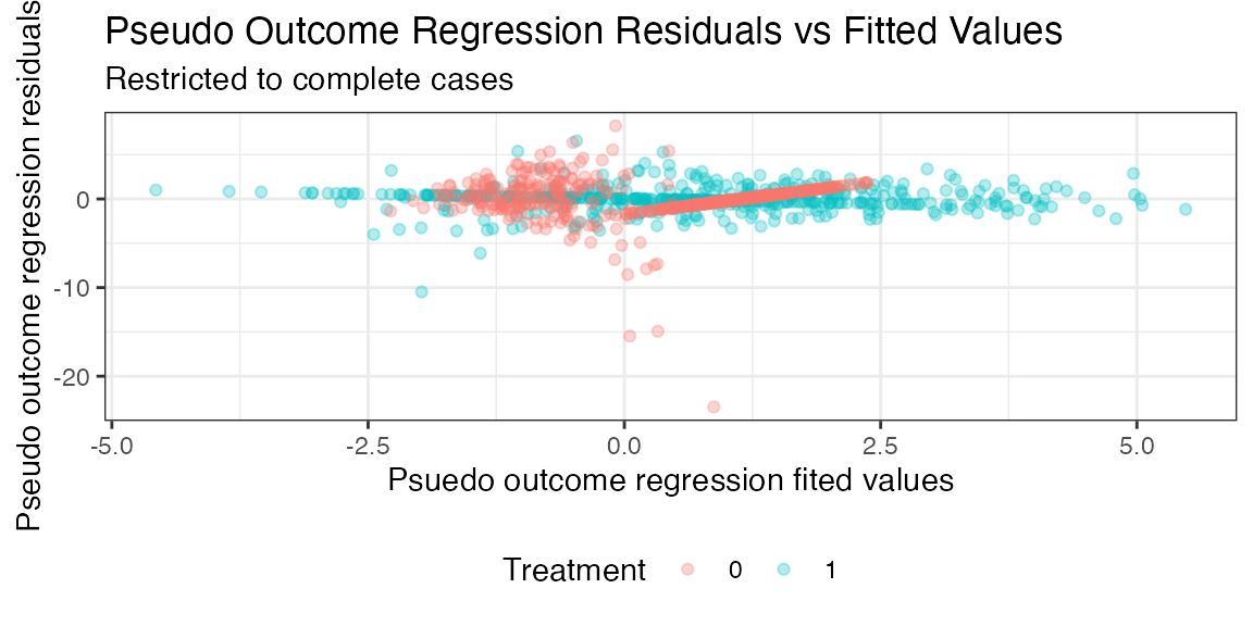

Alternatively, users can cycle through all diagnostic plots by leaving the type argument unspecified or setting it to 'All'

plot(res)

Technical Details

Observed and full data influence functions

drcmd leverages developments from semiparametric theory for the estimation of functionals in the presence of missing data. Key to semiparametric efficient estimation with missing data is the conceptualization of (i) the full-data distribution one would have access to in the presence of missing data, and (ii) the observed data distribution one actually has access to. In full generality, suppose there exists a missingness free distribution one would ideally sample observations $F_i$ from the full-data distribution $\mathbb{P}_F$: $$F_i \sim \mathbb{P}_\text{F}, \ \ \ \ i=1,\ldots,n,$$ where interest lies in some pathwise differentiable statistical functional $\Psi(\mathbb{P}_\text{F})$ and $F_i$ can be decomposed into $F_i = (V_i, U_i)$.

Rather than observe data from $\mathbb{P}_F$, we instead observe data from the observed-data distribution $\mathbb{P}_O$ containing i.i.d. observations $$O_i = (W_i, \ V_i, \ R_i U_i, \ R_i)\sim \mathbb{P}_O.$$ Above, $U_i$ is only observed when $R_i=1$, and $W_i$ is observed for all $i$ and contains variables that are (i) possibly predictive of missingness, and (ii) but not a component of $F$, in the sense that they wouldn’t be used for estimating the target estimand when one has access to complete data. $W$ is closely connected to the notions of proxy and surrogate variables.

Letting $\chi(O, \mathbb{P}_\text{F})$ denote the efficient influence curve for $\Psi(\mathbb{P}_\text{F})$, the efficient influence curve for $\Psi(\mathbb{P}_\text{F})$ induced by the observed data distribution can be written $$\chi(O,\mathbb{P}_O) = \frac{R}{\kappa(Z)}\chi(F,\mathbb{P}_\text{F}) - \left(\frac{R}{\kappa(Z)} - 1 \right) \varphi(O)$$ where $\varphi(O) = \mathbb{E}[\chi(O,\mathbb{P}_\text{F}) | Z]$ and $\kappa(Z) = \mathbb{P}(R=1|Z)$. The above representation holds so long as the missing at random assumption $U \perp R | Z$ holds, where $Z = (W, V)$ collects all variables which are always observed.

Estimation of counterfactual means

Throughout, we will consider the scenario of estimating a generic counterfactual mean $\mathbb{E}[Y(a)]$. Under the core causal inference assumptions of consistency, positivity, and exchangeability, the counterfactual mean can be expressed as $$\mathbb{E}[Y(a)] = \psi_a := \mathbb{E}[m_a(X)]$$ where $m_a(X) = \mathbb{E}[Y|A=a,X]$ and $\psi_a$ is identified under the complete-data distribution.

To build intuition, return to the earlier outcome proxy example where we observe $$O_i = (R_i Y_i, A_i, X_i, Y_i^*) \sim \mathbb{P}_O$$ and assume $Y \perp R | A, X, Y^*.$ In this setting, the ideal distribution is given by $F = (Y, A, X)$, and notice $W=Y^*$, $Z = (Y^*, A, X)$ and $U = Y$. It’s well-known that the efficient influence curve for $\psi_a$ under the full-data distribution is given by $$\chi(F, \mathbb{P}_F) = m_a(X) + \left( \frac{I(A=a)}{\mathbb{P}(A=a|X)} \right) \left( Y - m_a(X) \right) - \psi_a$$ In turn, the observed data EIC, a crucial ingredient for constructing efficient semiparametric estimators, is given by

$$\begin{aligned} \chi(F, \mathbb{P}_O) &= \frac{R}{\kappa(Z)}\chi(F,\mathbb{P}_\text{F}) - \left(\frac{R}{\kappa(Z)} - 1 \right) \varphi(O) \\ &= \frac{R}{\kappa(Z)}\left\{ m_a(X) + \left( \frac{I(A=a)}{\mathbb{P}(A=a|X)} \right) \left( Y - m_a(X) \right) - \psi_a \right\} - \left(\frac{R}{\kappa(Z)} - 1 \right) \varphi(O) \end{aligned}$$

We now consider numerous means by which $\hat \psi_a$ can be estimated.

Plug-in estimator

Recalling $m_a(X) = \mathbb{E}[Y|A=a,X]$, one can construct a plug-in estimator of $\psi_a$ of the form

$$\hat \psi_a = \frac{1}{n} \sum_{i=1}^n \hat{m}_a(X_i)$$ above, $\hat m_a(X)$ can be estimated through a regression of $Y$ on $A$ and $X$ which weights the underlying loss function by $R/\hat \kappa(Z)$, where $\hat \kappa(Z)$ are estimated complete case probabilities. In the event that covariates are partially missing, one can instead implement the plug-in estimator

$$\hat \psi_a = \frac{1}{n} \sum_{i=1}^n \left(\frac{R_i}{\hat{\kappa}(Z_i)} \right) \hat{m} \ {}_a(X_i)$$

While the above estimator is straightforward to implement, its asymptotic distribution is intractable when the above nuisance functions are estimated with machine learning methods. Specifically, it can be shown that under modest regularity conditions,

$$\hat \psi_a - \psi_a = \frac{1}{n} \sum_{i=1}^n \chi_a(O_i; {\mathbb{P}}_O) - \mathbb{E}\left[ \chi_a(O_i; \hat{\mathbb{P}}_O) \right]+ o_p(n^{-1/2})$$ where $\chi_a(O_i; \hat{\mathbb{P}}_O)$ is the efficient influence curve for $\psi_a$ under the observed data distribution. The term $\mathbb{E}\left[ \chi_a(O_i; \hat{\mathbb{P}}_O) \right]$ above is crucial, as it is typically of a slower order than $n^{-1/2}$, invalidating standard asymptotic inference and making the construction of confidence intervals an intractable task. In turn, $\mathbb{E}\left[ \chi_a(O_i; \hat{\mathbb{P}}_O) \right]$ is typically referred to as a plug-in bias term. drcmd allows for estimators based on two general frameworks that aim to remove this plug-in bias: one-step estimation and targeted maximum likelihood estimation.

One-step estimation

The default estimation method used by drcmd is based on the method of one-step bias correction. The one-step estimator simply removes the above plug-in bias by adding its estimate back on to the plug-in:

$$\hat \psi_a^\text{OS} = \hat{\psi}_a + \frac{1}{n} \sum_{i=1}^n \chi_a(O_i; \hat{\mathbb{P}}_O)$$ implying the form

$$\hat \psi_a^\text{OS} = \hat \psi_a^\text{PI} + \frac{1}{n} \sum_{i=1}^n \left[\frac{R_i}{\hat \kappa(Z_i)}\left\{ \hat m_a(X_i) + \left( \frac{I(A_i=a)}{\hat{\mathbb{P}}(A_i=a|X)} \right) \left( Y_i - \hat m_a(X_i) \right) - \hat{\psi}_a^\text{PI} \right\} - \left(\frac{R_i}{\hat \kappa(Z_i)} - 1 \right) \hat\varphi(O_i)\right]$$

Empirical efficiency maximization (EEM)

The nuisance function $\varphi(O)$, often referred to as the pseudo-outcome regression function, is an inherently complicated nuisance function:

$$\varphi_a(O) = \mathbb{E}\left[ m_a(X_i) + \left( \frac{I(A_i=a)}{{\mathbb{P}}(A_i=a|X)} \right) \left( Y_i - m_a(X_i) \right) - \psi_a \bigg| \ Z \ \right]$$ where $Z$ collects all non-missing variables. Particularly when the relative share of complete cases $P(R=1)$ is small, estimation of $\varphi_a(O)$ can be a difficult task. The empirical efficiency maximization framework is motivated by the finding that (under standard regularity conditions),

$$\hat \psi_a - \psi_a = O_\mathbb{P}\left( \frac{1}{\sqrt n} + ||\hat m_a - m_a|| \cdot ||\hat g_a - g_a|| + ||\hat \kappa - \kappa || \cdot ||\hat \varphi_a - \varphi_a|| \right),$$ meaning that if the complete case probabilities $\kappa(Z)$ are estimated consistently, mis-specification of $\varphi_a$ will not influence bias of the estimator, but will hamper efficiency.

Targeted maximum likelihood estimation

Recalling the form of the observed data influence curve,

$$\chi(O; \mathbb{P}_O) = \frac{R}{\kappa(Z)}\chi(F,\mathbb{P}_\text{F}) - \left(\frac{R}{\kappa(Z)} - 1 \right) \varphi(O),$$ the targeted maximum likelihood approach aims to remove the above plug-in bias by updating the initial estimates $\hat \kappa(Z)$ and $\hat m_a(X)$ in a manner where

1. The updated estimate $\hat \kappa^*(Z)$ is set so that $$\begin{equation} \label{eq:tml-1} \frac{1}{n} \sum_{i=1}^n \left(\frac{R_i}{\hat \kappa(Z_i)^*} - 1 \right) \hat{\varphi}(O_i) = 0 \end{equation}$$
2. Using the updated $\hat{\kappa}^*(Z)$, the updated plug-in estimate $\hat{m}_a^*(X)$ is set so that $$\begin{equation} \label{eq:tml-2} \frac{1}{n} \sum_{i=1}^n \left\{\frac{R_i}{\hat \kappa(Z_i)^*} \right\}\left(\frac{I(A_i=a)}{\hat g_a(X_i)} (Y_i - \hat m_a^*(X_i) )\right) =0 \end{equation}$$

The final $\hat{m}_a^*(X_i)$ is used to construct the final plug-in estimator

$$\hat{\psi}_a^\text{TMLE} = \frac{1}{n} \sum_{i=1}^n \hat m_a^*(X_i)$$

and in the case where the covariates are partially missing, the final plug-in estimator is given by

$$\hat{\psi}_a^\text{TMLE} = \frac{1}{n} \sum_{i=1}^n \left(\frac{R_i}{\hat \kappa(Z_i)^*} \right) \hat{m}_a^*(X_i)$$

Critically, () and () above imply that the plug-in bias of $\hat \psi_a^\text{TMLE}$ is zero, allowing for the same asymptotic analysis enjoyed by $\hat \psi_a^\text{OS}$. TML additionally guarantees its resulting parameter estimates will respect the bounds of the parameter space.

Standard error estimation

For all estimands in drcmd, standard error estimation is based on asymptotic variance formulae.

Counterfactual means: Let $\hat \psi_a$ be an estimator of $\psi_a = \mathbb{E}[Y(a)]$, based on the observed data influence curve $\chi_a(O,\eta)$, where $\eta$ collects all nuisance functions and $\mathbb{E}[\chi_a(O,\eta)]=0$. It can be shown under modest regularity conditions on the estimation rates of all nuisance functions that $$\hat \psi_a - \psi_a = \frac{1}{n} \sum_{i=1}^n \chi_a(O_i, \eta) + o_p(n^{-1/2})$$ In turn, the asymptotic variance of $\hat \psi_a$ is given by $\mathbb{E}[ \chi_a(O,\eta)^2]$. Standard error estimates are obtained by plugging in the empirical influence curve $\hat \chi_a(O,\hat \eta)$ for $\chi_a(O,\eta)$: $$\sqrt{\ \frac{1}{n} \sum_{i=1}^n \chi_a(O_i, \hat \eta)^2\ }$$

Risk ratio: Let $\hat \psi_1$ and $\hat \psi_0$ be asymptotically linear estimators of $\psi_1$ and $\psi_0$, respectively, and let $$\Sigma = \begin{pmatrix} \sigma_1^2 & \nu \\ \nu & \sigma_0^2 \end{pmatrix}$$ be the asymptotic covariance of $\hat \psi_1$ and $\hat \psi_0$. A straightforward application of the multivariate delta method implies the asymptotic variance of the risk ratio estimator $\hat \psi_1/\hat \psi_0$ is given by
$$\begin{aligned} \nabla g^\top \Sigma \nabla g \end{aligned}$$ where $\nabla g = (1/\psi_0, -\psi_1/\psi_0^2)$ is the gradient of $g(\psi_1,\psi_0) = \psi_1/\psi_0$. Evaluating the above expression yields $$\begin{aligned} \frac{\sigma_1^2}{\psi_0^2} + \frac{\sigma_0^2 \psi_1^2}{\psi_0^4} - \frac{2\nu \psi_1}{\psi_0^3}. \end{aligned}$$drcmd estimates the above asymptotic variance by substituting plug-in estimates for each component.

Odds ratio: Continue to let $\hat \psi_1$ and $\hat \psi_0$ be asymptotically linear estimators of $\psi_1$ and $\psi_0$, respectively. One can (i) find the asymptotic variance of the log odds ratio estimator $\log(\hat \psi_1/\hat \psi_0)$, and (ii) apply the delta method an additional time to obtain the asymptotic variance of the odds ratio estimator $\hat \psi_\text{OR} = \hat \psi_1/(1-\hat\psi_1) \big/\hat \psi_0 /(1-\hat \psi_0)$:

$$\begin{aligned} \psi_\text{OR}^2 \left( \frac{\sigma_1^2}{\psi_1^2(1-\psi_1)^2} + \frac{\sigma_0^2}{\psi_0^2(1-\psi_0)^2} - \frac{2\nu}{\psi_1(1-\psi_1)\psi_0(1-\psi_0)} \right). \end{aligned}$$

References

Kennedy, Edward H. 2022. “Semiparametric Doubly Robust Targeted Double Machine Learning: A Review.” arXiv Preprint arXiv:2203.06469.

Robins, James M, Andrea Rotnitzky, and Lue Ping Zhao. 1994. “Estimation of Regression Coefficients When Some Regressors Are Not Always Observed.” Journal of the American Statistical Association 89 (427): 846–66.